Relief Well Operations
Initial Relief Well Planning
Relief well planning was started as a contingency immediately after the blowout occurred with full resources directed to that effort after the second drillpipe kill attempt failed. These "design process" steps, in generic terms are the following: defining relief well objective, defining kill point(s), defining hydraulic communication method, evaluate position uncertainty, evaluate geology, define attack angle, develop an electromagnetic ranging strategy, determine surface location(s), develop relief well trajectory, define relief well casing program, define survey program, evaluate kill hydraulics, determine the number of relief wells, define kill equipment, and project refinement for drilling and kill. The figure below outlines the relief well planning process that was followed.
Ramp-up to an Incident Command Type of Organization
 After the decision was made to drill
relief wells to control the blowout it was necessary to ramp-up to an Incident Command
(ICS) type organization to efficiently manage the project which would last for at least 2
months. The chart on the left illustrates the basic organization that was utilized
for the project. John Wright was the project leader for relief well operations.
After the decision was made to drill
relief wells to control the blowout it was necessary to ramp-up to an Incident Command
(ICS) type organization to efficiently manage the project which would last for at least 2
months. The chart on the left illustrates the basic organization that was utilized
for the project. John Wright was the project leader for relief well operations.
Source Control – Relief Well Branch
The Relief Well Branch sub units are shown in more detail below. The routine drilling services are coordinated by a designated Drilling Rigs Group Leader. The logical choice for this position is a Senior Drilling Engineer (supported by the Drilling Superintendent as required). This is a functional position and would be filled by the Senior Drilling Engineer assigned initially to the Relief Well Planning Task Force. In this position he will be responsible for assisting the Special Services Group, initially, in planning the relief well standard drilling program (e.g., casing design, wellheads, cement, drilling mud, bits, etc.). After the relief well is spudded he will coordinate all normal drilling activities between the relief well rig(s) and support the special services unit at the rig site. The Drilling Supervisor will be the Unit Leader for his rig. He will maintain most of his normal responsibilities during the drilling of the relief well. This will include all normal drilling operations, cementing, casing, logistics including well control and emergency response. If there is a well control emergency on the relief well it will be his responsibility to carry out appropriate response actions (the relief well special services unit leader will provide emergency response guidelines before drilling begins).
Special Relief Well Services performed at the rig will be planned and supervised by either the Kill Unit Leader or the Intersection Unit Leader. The Intersection Unit Leader will be responsible for making the intersection at the chosen kill point. He will supervise the directional drilling, surveying (surface and borehole), and the homing-in services. He will coordinate closely with the Rig Supervisor and the Drilling Rigs Unit Leader to minimize mis-communication (the Intersection Unit Leader will have final decision on field procedures, for these services, if there are conflicts between service company personnel). The Intersection Unit Leader has three functional Task Force positions under him. They are: Directional Drilling Task Force Leader, Surveying Task Force Leader and a Homing-in Task Force Leader. These positions may or may not all be filled depending on the scope and the number of the relief wells drilled.
The Kill Unit Leader will plan, coordinate and supervise: (1) the high pressure pumping plant design; (2) low pressure kill mud pumping, storage and transfer; (3) kill fluid design including any reactive chemicals or polymers usage; (4) obtaining hydraulic communication between the relief well and the blowout; (5) the kill pumping operations; (6) kill monitoring and diagnostics during pumping; (6) plug and abandonment. The Kill Unit Leader has five functional Task Forces under his supervision. These are: High Pressure Pumping; Low Pressure Pumping/Mud Storage and Transfer; Kill Fluids; Kill Cementing; and Kill Modeling and Diagnostics. These positions may or may not all be filled depending on the scope of the kill operations and the number of the relief wells drilled.
Relief Well Branch- Special Services - Intersection Unit
 The Special Services -
Intersection Unit is shown in more detail in the org-chart on the left. The Special
Services Group Leader acts as the special services project manager for the relief well. He
will coordinate the Daily Planning Cycle, Incident Action Plans, the development of the
General Plan and supervise its execution through the intersection, kill and P&A.
The Special Services -
Intersection Unit is shown in more detail in the org-chart on the left. The Special
Services Group Leader acts as the special services project manager for the relief well. He
will coordinate the Daily Planning Cycle, Incident Action Plans, the development of the
General Plan and supervise its execution through the intersection, kill and P&A.
The Kill Unit Leader and the Intersection Unit Leader Positions are functional. The Special Services Unit Leader may fill one, both or neither of these positions depending on the scope of the kill operations and the number of the relief wells drilled and his personal experience.
The Intersection Unit Leader is a specialist in relief well type intersections with experience in all aspects of trajectory planning, directional drilling, surveying and homing-in. He is responsible for planning and supervising all intersection operations.
Below the Intersection Unit Leader are three functional Task Forces. One for Directional Drilling, one for Surveying and one for Homing-in. These units each have a Unit Leader positions. Someone must perform the function but they may or may not be separate individuals (e.g., the Intersection Unit Leader may also take on the Survey and Homing-in Task Force Leader positions). The size and critical nature of the project will dictate the filling of these positions with dedicated individuals.
The Directional Task Force Leader is a specialist in precision directional drilling peculiar to well intersection and homing-in requirements. Responsible for well placement as per plan, he will coordinate the directional drilling activities of the service company. This is best done through the contractors directional drilling coordinator. If he is not available on a full time basis, the Task Force Leader will work directly with the DDS for each rig.
The Surveying Task Force Leader will coordinate all the surveying activities through the service company to include: MWD, drop magnetic multishots and gyros. He is a specialist in borehole position uncertainty and QA/QC of the surveying instruments being used. He is responsible for survey accuracy in the blowout and all relief wells. The coordination is best done through the contractor’s MWD and survey coordinator. If this person is not available full time he will coordinate directly with the operators.
The Homing-in Task Force Leader is a specialist in casing detection tools, their application and QA/QC of data. He will coordinate with the homing-in service company to design the ranging depths, procedures, relative well trajectories and uncertainty of calls. This position is again functional and might be filled by the Survey Task Force Leader or the Intersection Unit Leader if they are qualified.
Relief Well Branch- Special Services - Kill Unit
 The Kill Unit is shown in more
detail in the orgchart on the left. The Kill Unit Leader is an engineering specialist in
planning, preparing for and directing the kill operation from either the surface or from a
relief well. The Kill Unit is shown as a single group for both Surface Control and Relief
Well as it is not common for both teams to work simultaneously on both (there generally is
not enough resources, equipment or personnel, to set up kill spreads on two relief wells
and a surface kill operation simultaneously). Kills are usually planned in sequences
(e.g., if a surface kill is possible, several attempts may be tried before resorting to
the relief wells). It may be necessary, however, in cases where drilling is fast, that
separate task forces may have to mounted.
The Kill Unit is shown in more
detail in the orgchart on the left. The Kill Unit Leader is an engineering specialist in
planning, preparing for and directing the kill operation from either the surface or from a
relief well. The Kill Unit is shown as a single group for both Surface Control and Relief
Well as it is not common for both teams to work simultaneously on both (there generally is
not enough resources, equipment or personnel, to set up kill spreads on two relief wells
and a surface kill operation simultaneously). Kills are usually planned in sequences
(e.g., if a surface kill is possible, several attempts may be tried before resorting to
the relief wells). It may be necessary, however, in cases where drilling is fast, that
separate task forces may have to mounted.
The Kill Unit is further divided into specific functional Task Forces. These Task Forces may or may not require dedicated Leaders depending on the circumstances and scope of the kill job (i.e., the Kill Unit Leader may fill one or more of the Task Force Leader positions). The Task Force functions are:
 The Source Control - Planning
Section is shown in more detail in the orgchart on the left. The Planning Section
for Source Control operates slightly different from the ICS described Planning Section for
say an oil spill or other disaster. In those cases the Planning Section plans what the
Operations Section is going to do on a daily and long-range basis. This is done by setting
objectives but not tactics on how to accomplish those objectives.
The Source Control - Planning
Section is shown in more detail in the orgchart on the left. The Planning Section
for Source Control operates slightly different from the ICS described Planning Section for
say an oil spill or other disaster. In those cases the Planning Section plans what the
Operations Section is going to do on a daily and long-range basis. This is done by setting
objectives but not tactics on how to accomplish those objectives.
Due to the rare occurrence of blowout source control operations and the requirement to utilize both blowout specialists and local personnel in much of the planning as well as operations, this format needs to be modified. The Planning Section, in reality, turns out to be more of an engineering/technical support section. The blowout engineering specialists will develop a control strategy for both surface and relief well options and the Planning Section will provide local engineering technical support to turn the strategy into an acceptable design and then assist in the daily planning and implementation cycle as required. Most of the support engineering staff will only be required during the initial planning cycle and will not be full time members of the Source Control Team.
The Engineering/Technical Support Unit Leader is logically a Qualified Individual from Drilling Engineering, e.g., the department supervisor. Under his direction (supported by blowout engineering specialists) will be five functional Task Forces as required by the circumstances: (1) Surface Engineering Support; (2) Relief Well Engineering Support; (3) Situation, Status and Documentation Support; (4) Blowout Diagnostics and Kill Engineering Support; (5) Risk Assessment and Management Support.
The Surface Engineering Support Task Force Leader would be a Senior Drilling Engineer if the blowout was on a MODU or a Production Operations Manager for the affected platform if a platform blowout. He would be responsible for coordinating engineering personnel as required to support the Surface Control Operations. He would be advised by the blowout engineering specialists and liaison closely with operations.
The Relief Well Engineering Support Task Force Leader would be a Senior Drilling Engineer. He would be responsible for coordinating engineering personnel as required to plan and support the relief well. He would be advised by the blowout engineering specialists and would take over as the MODU Group Leader after the relief wells are spudded.
The Blowout Diagnostics and Kill Engineering Support Task Force Leader would logically be a Petroleum Engineering Manager in the area where the blowout is located. He will work with the blowout specialists to determine the blowout characteristics (e.g., flow rate, flow path, pressures, GOR, IPR, chokes, uncertainties, sensitivities, geologic constraints, kill hydraulics, etc.).
The Situation, Status and Documentation Task Force Leader may be a Qualified Individual from data management or perhaps a drilling engineer. He would be responsible for supplying personnel with documentation skills to provide daily situation and status reports, document collection and archival, and documentation support for the functional groups as required.
The Risk Assessment/Management Task Force Leader would logically be the Loss Prevention Manager. He would be responsible for responders health and safety, evaluating risk based on safety, environment, asset damage, and operations/economics. He may activate specialists in risk assessment (e.g., hydrocarbon ignition specialists, environmental impact specialists, etc.).
All positions are functional and would be activated only if required and deactivated when no longer needed.
Combining data from the two surface kill attempts, the pressure temperature log run in the blowout drillpipe, reservoir pressure data obtained from offset wells, oil recovery and all other geologic and drilling information available the hydraulic kill team defined possible blowout scenarios. These scenarios were evaluated utilizing computer simulators for sensitivities to hydraulic kill requirements. The worst plausible scenario was used for design.
The Flowpath was assumed unrestricted with an average open hole diameter of 14". The exit point was at 105 m with no choking affect. The oil flowrates were relatively insensitive to kill hydraulics and could vary from 40 to 90 MMscf/d. The gas rates were estimated at 500 MMscf/d. The worst plausible loss rates into the fracture system after the flow was stopped was considered to be as high as 30 bpm, however, it potentially could be higher. It would take 60 days to complete the relief wells during which time the gas rate would drop nearly in half.
Relief Well Kill Objectives.
Relief wells can be used in several ways to control a blowout. These are usually divided into two categories: (1) direct intersection with the wellbore followed by: heavy mud kill (primarily mass flow); dynamic kill (friction + mass flow); reactive fluid kill (kill fluid reacts with blowout fluid or two kill fluids are injected); polymer kill (polymers are designed to gel in the blowout wellbore); or relief well production. (2) relief well is drilled into the flowing reservoir followed by: reservoir flood with water, brine and/or polymer; or relief well production.
The killing of a blowout with a relief well is normally planned in three parts. First the hydrocarbon flow must be stopped. This may be done with any of the described methods depending on the circumstances. Second the kill must be transition from a dynamic state to a static state without the flow restarting. And third, the well must be permanently plugged to prevent the flow from restarting sometime in the future.
Direct intersection is generally preferred over reservoir flooding techniques if that option is possible and was chosen as the primary method followed by a mass flow hydraulic kill. The consequences for failure to kill the blowout were so high that secondary contingencies were also made. They were: (1) If the mass flow kill was unsuccessful then reactive kill fluids would be used to plug the flow path. This would require two conduits. (2) A reservoir flood well would be planned if hole diameters were much larger than predicted and sufficient volume of fluids could not be pumped into the direct intersections to either mass flow kill or plug-off the flow path.
Number of Relief Wells.
Three (3) relief wells would be planned and drilled. The risk assessment phase of the relief well planning determined that no chance of failure should be taken. To accomplish this, two intersection wells would be planned, so reactive fluids could be pumped if the hydraulic kill was unsuccessful. A third well would also be planned as a reservoir flood to act a contingency to the intersect wells. The flood well, however, was not designed to kill the blowout alone but to assist the intersect well(s) by reducing the flow rate.
Relief Well Intersection Depths
 Many factors, both drilling and kill related, must be evaluated in
an iterative fashion to determine the optimum intersection depth. On the drilling side
these include: surface location, relative position uncertainty, blowout trajectory,
borehole intersection constraints, ranging constraints, drilling equipment constraints,
geologic and well control constraints. On the kill side they include: method of hydraulic
communication, blowout scenario, kill fluids, relief well construction, geologic
constraints, ability to transition to a static kill and plug and abandon the blowout.
Many factors, both drilling and kill related, must be evaluated in
an iterative fashion to determine the optimum intersection depth. On the drilling side
these include: surface location, relative position uncertainty, blowout trajectory,
borehole intersection constraints, ranging constraints, drilling equipment constraints,
geologic and well control constraints. On the kill side they include: method of hydraulic
communication, blowout scenario, kill fluids, relief well construction, geologic
constraints, ability to transition to a static kill and plug and abandon the blowout.
Based on this criteria, the intersection points for the blowout were evaluated as follows: (1) Relief well 1, would intersect the open wellbore between 2750 and 2800 m tvd and Relief well 2, between 2800 and 2850 m tvd (attempt to keep separation between intersection points between 25 and 50 m. This depth was: in the near vertical section of the blowout, < 2�; sufficient to accomplish a hydraulic kill and also allow reactive fluids to be mixed in the blowout wellbore by pumping down both of the relief wells. The intersection relative attack angle would be between 5� and 10�. (2) The flood relief well would be positioned at a relative distance between 10 and 15 m from the blowout at the top of the producing reservoir.
Method of Gaining Hydraulic Communication.
The primary method for the intersection wells would be direct intersection with a bit. The secondary method would be to acidize if the relative proximity between the boreholes was 1 m or less. The flood well would gain communication by pumping water at below the fracture gradient of the reservoir. Polymer would be used to help direct the flow to the blowout.
Geologic Considerations. The formations to be drilled consisted of: a surface sand layer down to approximately 200 m; a section of thick anhydrites, salts and claystones down to approximately 1100 m; open marine lime mudstones down to approximately 2900 m; a marine cherty limestone down to approximately 2960 m; a section of weathered volcanics and claystones to the top of the reservoir at approximately 3025 m. The reservoir consists of fine-medium sand/sandstone with the GOC at approximately 3050 m.
 The first consideration was to evaluate
potential shallow gas charging along the proposed relief well path. This was considered
low as the P/T log indicated the flow path to be exiting the blowout casing at 105 m in
the porous surface sands. Since the crater and was relieving the pressure to the
atmosphere it was unlikely shallow surface aquifers were being charged. There were
fractures in the lime mudstones predicted in the north-south plane but the flowing
pressure in the borehole was lower than pore pressure and did not present a charging
threat.
The first consideration was to evaluate
potential shallow gas charging along the proposed relief well path. This was considered
low as the P/T log indicated the flow path to be exiting the blowout casing at 105 m in
the porous surface sands. Since the crater and was relieving the pressure to the
atmosphere it was unlikely shallow surface aquifers were being charged. There were
fractures in the lime mudstones predicted in the north-south plane but the flowing
pressure in the borehole was lower than pore pressure and did not present a charging
threat.
The limestone at the proposed intersection point was highly reactive to HCL acid and would facilitate communication if a direct intersection was not achieved. The cherty limestones would be avoided for precision directional drilling work. The claystones above the reservoir where highly reactive to water and would require casing off before starting a water flood. Temperature at the intersection point was less than 240� F and was not expected to cause any special drilling related problems.
 Position Uncertainty of the
Blowout. The blowout was drilled vertical down through the reservoir and
plugged back to 2831 m. The well was then kicked off with MWD and motor along an azimuth
of 240� using build rates of 8-12�/30m. The TD at the time of the blowout was 3212 m MD/
3100 m tvd with 76� inclination in the well. MWD was not used above the kick-off point of
2831 m with the definitive survey being a film based MMS. The instrument was re-checked
and the film re-read by 3 different surveyors. The position uncertainty assigned to the
blowout at the proposed intersection depth was � 15 m at a 3 sigma confidence level and
� 5 m at 1 sigma. The relative surface uncertainty of the blowout could be fixed with
optical/laser surveying techniques to less than 1 m.
Position Uncertainty of the
Blowout. The blowout was drilled vertical down through the reservoir and
plugged back to 2831 m. The well was then kicked off with MWD and motor along an azimuth
of 240� using build rates of 8-12�/30m. The TD at the time of the blowout was 3212 m MD/
3100 m tvd with 76� inclination in the well. MWD was not used above the kick-off point of
2831 m with the definitive survey being a film based MMS. The instrument was re-checked
and the film re-read by 3 different surveyors. The position uncertainty assigned to the
blowout at the proposed intersection depth was � 15 m at a 3 sigma confidence level and
� 5 m at 1 sigma. The relative surface uncertainty of the blowout could be fixed with
optical/laser surveying techniques to less than 1 m.
Homing In Strategy. Since a direct intersection into a 14" diameter hole is desired a method for "homing in" on the blowout from the relief well is required. Three commercial methods are available for this necessity require steel tubulars in the blowout well bore and the third requires access the blowout. The first is a passive "magnetostatic" technique that uses sensitive magnetometer arrays to look for perturbations in earth’s magnetic field caused by target tubulars. The second is an active "electromagnetic" technique that requires electric current to be placed on the target tubulars. This creates a radial magnetic field around the tubular that is sensed by a wireline tool in the relief well. The current may be applied either from a down hole electrode on the wireline tool or in some circumstances tied to the wellhead at the surface depending on the depth of interest. The third method uses a solenoid in the blowout well, assuming there is pipe in the blowout that can be accessed by a wireline. The solenoid produces a known magnetic field that is sensed from a wireline tool in the relief well.
 If possible the solenoid method is preferred as it
eliminates most of the limitations and uncertainties of the first two methods and has an
effective maximum range of ˜ 50 m. As the drillpipe in the blowout was accessible at
this time it was chosen as the primary method. It would take, however, 60 days to drill
the relief well and during that time access to the blowout could be lost either by: crater
movement swallowing the wellhead, drillpipe cut-off at the blowout exit point at 105 m, or
by fire. The secondary method would be the electromagnetic technique using downhole
current injection. This method has a range of 60 m under ideal conditions, however, this
case was not ideal. Non- conductive oil and gas was the only fluid flowing in the blowout
wellbore making the transfer of current onto the drillpipe uncertain. The estimated
effective range might be reduced by at least 50% or more worst case. Magnetostatic
techniques could also be used as a final option as the two well converged to less than 10
m.
If possible the solenoid method is preferred as it
eliminates most of the limitations and uncertainties of the first two methods and has an
effective maximum range of ˜ 50 m. As the drillpipe in the blowout was accessible at
this time it was chosen as the primary method. It would take, however, 60 days to drill
the relief well and during that time access to the blowout could be lost either by: crater
movement swallowing the wellhead, drillpipe cut-off at the blowout exit point at 105 m, or
by fire. The secondary method would be the electromagnetic technique using downhole
current injection. This method has a range of 60 m under ideal conditions, however, this
case was not ideal. Non- conductive oil and gas was the only fluid flowing in the blowout
wellbore making the transfer of current onto the drillpipe uncertain. The estimated
effective range might be reduced by at least 50% or more worst case. Magnetostatic
techniques could also be used as a final option as the two well converged to less than 10
m.
Initial Search Point. The items evaluated in establishing the initial casing search point were:
After evaluating the above criteria it was decided to start the search for the drillpipe approximately 200 m above the proposed intersection point at a minimum horizontal distance of 50 m to allow enough depth for course corrections. The predicted position uncertainty of the blowout is within the predicted range of the chosen homing-in methods, however, the relief well trajectory selected must be efficient to avoid high dog-legs. A bypass and plugback of the blowout drillpipe for triangulation purposes would be used only if necessary.
Planned ranging points. If the solenoid technique were used five (5) ranging runs were planned for relief wells 1 and 2 and two (2) for relief well 3. These would start at a horizontal distance of ˜ 50 m from the blowout with the remainder taken between this position and intersection at relative distances of approximately 1/2 of the previous.
If the downhole injection electromagnetic method was used seven (7) ranging runs were planned for relief wells 1 and 2 and two (2) for relief well 3. These would start at a horizontal distance of 50 m for relief well 1 and ˜ 40 m for relief well 2. A range would not be taken in relief well 2 if good data was not obtained at a similar distance in relief well 1. A solenoid would be run between relief well 1 and 2 to more accurately define their relative position to each other and to the blowout. A solenoid would also be run between relief well 2 and relief well 3 to fix relief well 3 to the blowout incase it was not possible to range on the blowout drillpipe from relief well 3 due to its trajectory planned for a water flood. Click here to see planned ranging zone of relief wells 1 and 2.
Relief Well Surface Locations. The items evaluated in choosing the surface location were:
Prevailing winds. Prevailing winds were predominately from the north west, however large variations in direction could occur over a short time period.
Surface hazards or obstacles. The only significant surface hazard was the oil flow path from the crater and the evacuation lagoons. The natural topography of the area around the crater allowed the oil to flow primarily to the west with a smaller amount flowing to the north before turning west. Bund walls were built to contain the flow approximately 300 north and 400 m west from the crater. Three oil evacuation lagoons were located ˜ 300 m to the south west. Two of the lagoons were connected to the crater by the surface flow of oil, the third was a fire safe lagoon located ˜ 75 south of the second and connected by underground pipelines. If a fire were to occur the relief wells should be located a safe distance from the oil lakes.
Toxic gases, heat radiation, noise, smoke. There was no H2S in the gas, heat radiation estimates made on 40 Mbopd and 400 MMscf/d estimated 300 m would be a sufficient distance from the crater. Noise was not considered as the flow was from a crater and noise level from the diverters was not substantial. Smoke was considered to be a problem due to large amounts of oil being burned in a crater. Experience from Kuwait indicated that 500 m should be a sufficient distance for most wind conditions.
Geological hazards or obstacles. Even though no supercharging was expected there were formations down to 1300 m with leached or fractured porosity. To be absolutely safe all relief wells would be drilled vertical until that depth. This would affect the maximum distance that the target could be reached without using extreme dog-legs. There was also potential for north south fractures in the limestone in the ranging zone. Approaching those fractures from 90� (i.e., from the west) would reduce formation noise during electromagnetic ranging.
 Well trajectory considerations. The blowout was vertical
at the intersect depth so those relief wells are not affected by blowout trajectory. The
flood well would target the blowout in the reservoir which was approximately 40 m west of
the wellhead with 76� inclination. It was desired to keep the average dog-leg severity in
the relief wells to < 5�/30 m in the upper section of the hole. This combined with the
50 m proximity 300 m above the intersection point and a kick-off no shallower than 1300 m
would limit the maximum distance from the wellhead for the relief wells.
Well trajectory considerations. The blowout was vertical
at the intersect depth so those relief wells are not affected by blowout trajectory. The
flood well would target the blowout in the reservoir which was approximately 40 m west of
the wellhead with 76� inclination. It was desired to keep the average dog-leg severity in
the relief wells to < 5�/30 m in the upper section of the hole. This combined with the
50 m proximity 300 m above the intersection point and a kick-off no shallower than 1300 m
would limit the maximum distance from the wellhead for the relief wells.
Using the above criteria three surface locations were chosen at an average of 750 m north of the blowout wellhead.
Relief Well Trajectories
Relief wells 1 & 2 were planned as a pair, both
utilizing a build, hold, drop/turn trajectory to align to their respective intersection
points with approximately 200 m of hold for alignment purposes during ranging. The planned
inclination for both final approach to target was 8� � 3�. The approach azimuth was
planned so that relief well 1 and 2 would converge at approximately a 90� relative
azimuth to each other (105� for RW1 and 195� for RW2. This was planned to allow for
triangulation between the relief wells and the blowout as the distance uncertainty of the
ranging tools was estimated to be larger than the relative azimuth uncertainty.
Click here to see vertical section view of relief
wells 1 and 2.
Relief Well 3, was planned to be a back-up to relief well 2, down to the 9-5/8" casing setting depth, if it were delayed extensively due to drilling or other problems. At the 9-5/8" setting depth it could proceed as an intersect well or turn and build to its primary flood target in the reservoir.
Relief Well 1. Relief Well 1 (Well 124), is planned vertical to KOP at 1300 m. Build at 3�/30m to 43� inclination at an azimuth of 153�. Hold to 2085 m tvd then drop & turn at 2�/30m to range 1 (50 m proximity to the blowout) at 2480 m tvd with 14� inclination and 133� azimuth. Based on the ranging results continue to drop & turn to range 2 at 2535 m tvd and so on to the next ranging point. The inclination and azimuth should basically be lined out at ˜ 8� and ˜ 105� respectfully at ˜ 2490 m tvd. Intersection is planned at approximately 2800 m tvd.
Relief Well 2. Relief Well 2 , was planned vertical to KOP at 1350 m. Then build at 3�/30 m to 41� inclination and 187.5� azimuth. Hold to 2115 m tvd then drop and turn at 2�/30m to 8� inclination and 195� azimuth at 2620 m tvd. This is also the 9-5/8" casing point and the first planned ranging point for this well. This basic inclination and azimuth will be maintained, depending on ranging results, until intersection is made at ˜ 2845 m tvd.
Relief Well 3. Relief Well 3 (flood well), was planned vertical to KOP at 1670 m. Then build to 43� inclination and 207� azimuth at 3.5�/30m. Hold to 2400 m tvd then drop and turn to 17.5� inclination and 242� azimuth at 2714 m tvd. This attitude would be held to the target in the top of the reservoir at ˜ 3026 m tvd. Click here to see traveling cylinder view of relief wells 1 and 2.
Casing Programs.
While conventional casing design criteria are employed when designing a relief well, several additional considerations must be investigated. The first is to design the kill string diameter to assure the control fluids could be pumped at the required rate without excessive surface pressure.
The second, if possible, is to allow for at least one additional emergency casing string to assure the required kill string diameter can be set. A third is to establish strength requirements for the casing strings that might be exposed to higher than normal burst and collapse forces during kill pumping, well control or complete loss of circulation.
A fourth is environmental considerations, such as hydrogen embrittlement on high strength casing and connections, casing wear, high dogleg considerations for bending stresses, thermal loading and temperature effects during kill operation (e.g., cold fluid being pumped down a hot well at high rates will cause high thermal tensile stresses).
The casing program for all three relief wells were planned the same down to the 9-5/8" shoe. Relief well 3, would additionally set a 7" liner to isolate reactive claystone formations just above the reservoir before starting the water flood. Relief wells 1 and 2 were planned to intersect with 8-1/2" open hole, however, a 7" liner was planned as a contingency if hole conditions prior to intersection required it.
The basic program consisted of:
Surveying Program. Due to uncertainty in the maximum range of the electromagnetic homing-in tools under the circumstances, the surveying criteria in all relief well scenarios would be critical. The proposed intersection scenarios required continuous steerable motor work in 3-D space kick-off to the intersection targets. This would require good quality control of the MWD data with cross checks made with north seeking gyros through the drillpipe and at casing points.
It was also extremely important to fix as accurately as possible the relative positions and elevations between the blowout wellhead and the relief wells. An independent true and magnetic north reference fix would also be made as opposed to accepting relative GPS references.
Surface Surveying
The objectives of the surface surveying were: (1) Define a true north relative bearing between each of the relief wells and the blowout wellhead. (2) Define a true north relative coordinate system between each of the relief wells and the blowout wellhead; and (3) Define the magnetic declination between true north and magnetic north at the blowout site.
The true north bearing would be established by setting two bench marks near one of the relief well sites separated by several hundred meters. Solar observations would then be made using precision optical theodolites during the morning and evening over a course of three days. These observations would then be used to determine the true north bearing between the two bench marks. Click here to see map.
The true north relative coordinate system would be defined by tying the two reference benchmarks back to a geographic control point located 23 km from the blowout site. The solar observations were used to confirm the origin bearings of the control point. With the bench marks fixed, the three relief wells were tied to the local net with x, y coordinates at the wellhead and z coordinate at the drill floor. The blowout wellhead was tied to the net using triangulation and affixing a prism on the wellhead. The final relative coordinates of all the wells with respect to a true north reference system was within a few centimeters.
Since drilling would be done with magnetic MWD instruments an accurate magnetic declination, inclination and total field strength was important model to eliminate any possibility of local field anomalies when comparing gyro surveys to magnetic derived MWD surveys. A MAG-01H Fluxgate Declinometer/Inclinometer would be used to cross check the IGRF computer models. The instruments consists of a 0.1 nT resolution single axis fluxgate magnetometer mounted on a Zeiss 020B steel free theodolite. This instrument would be set-up over the solar observation bench marks to: (1) measure the angle difference between magnetic north as measured by the Mag-01H and true north as measured by the solar observations; (2) Measure the magnetic inclination (dip angle); and (3) total magnetic field strength.
Magnetic Borehole Surveying.
The relief wells will be steered using MWD and cross checked with EMS surveys at predetermined depths. Magnetic survey data is gathered by Sperry Sun Drilling Services (SSDS). This includes MWD and EMS data. The data is stored in AHD, Gx, Gy, Gz, Bx, By, Bz with AHD in meters. Gx, Gy, Gz in G and Bx, By, Bz in micro Tesla. A rotational shot will be taken at the start of every bit run (however at least 30 m away from the casing shoe). A rotational shot should at least consists of 6 surveys at different toolface angles. A record of all BHAs used is kept including sensor positioning.
The magnetic field data to be used for magnetic survey data for all relief wells is:
The magnetic survey data would be processed using the Short Collar Solution program and RICE according to SSDC procedures using local Earth's magnetic field data (see above). At the end of a hole section drilled the survey data is again processed using quality control tolerances (see below). The processed survey data file shall be used as the definitive survey file.
If gravity field strength does not fall within its tolerances make sure that another measurement is performed with the tool held stationary . Incase magnetic field strength or dipangle do not fall within the tolerances, measure the Earth's field or check with BGS in Edinburgh. Quality control of Earth's magnetic field data may be accomplished by: 1) install a proton magnetometer to measure magnetic field strength on location. 2) Measure magnetic field strength with Barrington MAG 01H fluxgate on a weekly basis and to have regular contact with BGS in Edinburgh as per standard procedures to check on abnormal magnetic disturbances.
SSDS to perform BHA deflection calculations for every BHA using DIDRILL software program. The final survey data file has to be corrected for BHA deflection accordingly.
Gyro Surveying
Gyro surveying would be utilized to cross check the magnetic MWD data and to establish a very accurate survey from surface to the critical ranging zone. Gyrodata was the contractor, the instrument used was a 2" diameter north seeking gyro compass. Both drillpipe and casing surveys would be used. Drillpipe surveys would be used to quality control the MWD at the end of the tangent sections and potentially deeper if MWD accuracy is not considered sufficient to drill to the 9-5/8" casing point. Through drillpipe surveys would also be taken near the intersection point if magnetic interference is considered critical. Casing surveys would be made in 13-3/8" and 9-5/8" of all three relief wells.
Casing running procedures were as follows: Inrun: RIH taking surveys every 50 m till inclination of 30 deg. Perform a Mass Unbalance Offset measurement (5 readings). Continue inrun with 50 m intervals to TD.
Outrun: POOH with 10 m stations till maximum inclination of the well. Perform Mass Unbalance Offset measurement. Continue with outrun, 10 m intervals, till 13-3/8" casing point thereafter 25 m stations till surface.
Inclination difference between inrun and outrun should be less than 0.1 deg. Earth's rate of rotation tolerance is 0.08 deg/hr (equivalent to 2m lateral uncertainty at TD for wells 124,125 and 126). Nominal Earth's rate is 12.267 deg/hr.
Relief Well Kill Strategy
Hydraulic Kill Simulations. Well Flow Dynamics (using OLGA-WELL-KILL) were used to evaluate kill hydraulics utilizing one and two relief wells (independent and simultaneously) with various kill flow paths (i.e., pumping down annulus only or annulus and drillpipe) and casing configurations (7" liner or not).
The base case blowout data used for all simulations was:
The OLGA simulations using the base case scenario and no losses indicate a minimum of 85 bpm of 15 ppg mud and a volume of 2000 bbls would be required to stop the flow. If only one relief well was used the pump pressure would be 6000 psi, if both relief well annulus were used with 42.5 bpm on each, the pressure would be < 500 psi. The mud volume calculated is that amount required to stop the inflow. An additional 3 blowout hole volumes are required to circulate out gas if no losses are incurred.
A sensitivity was also evaluated to account for pressure drop in the reservoir between the planning phase and the actual kill date assumed 60 days later. The kill day reservoir pressure was estimated at 3410 psi resulting in a gas rate of 345 MMscf/d. The kill rate would reduce to 75 bpm of 15 ppg with an injection pressure of 3500 psi using a single relief well pumping down the annulus only.
Reactive Plug Design
Due to the uncertainty associated with a potential high loss rate, after a hydraulic kill was achieved, a reactive plug kill was designed as a contingency. This plug might be used to help stop the flow, stop the losses after a hydraulic kill was achieved or both. To apply these reactive fluids in the blowout wellbore at the intersection depth would require two independent flow paths. These paths included:
DOBC Gunk. A diesel oil bentonite cement gunk was designed utilizing a recipe of 150 ppb of cement grade Wyoming bentonite and 100 ppb of class "G" cement. The reology was pV = 24, YP = 119, gel = 56. DOBC gunk is relatively low in cost, it can be pumped at high rates in an annulus and large volumes can be readily mixed and stored (if the cement is added just before pumping). This mixture has practical reaction ratios between 2:1 to .25:1 DOBC gunk to 15 ppg mud. The best reaction was obtained with a 1/1 ratio setting to a dry paste in 20 to 45 sec depending on the shear rate (45 seconds if hand stirring and 22 seconds in a blender.
Based on the pilot test results the team decided to prepare a volume of ˜ 2500 bbls of DOBC gunk. The gunk would be injected down the annulus of the second relief well while mud was being injected down the annulus of the first. The maximum planned injection rate of gunk would be 40 bpm. Mud could be injected at rates up to 90 bpm. The combined maximum rate would be 130 bpm. The ratios would be kept between 0.33:1 to 1:1 gunk:mud.
Sodium Silicate-Cement: Sodium silicate and cement had been used in a similar blowout in 1993 to plug a flow after two surface hydraulic kill attempts had failed. A 40% solution of sodium silicate (density ˜ 11.4 ppg) was pilot tested with class "G" cement. Mixing ratios of 1:7 (silicate:cement) flash set in ˜ 30 seconds into a hard cement with compressive strength. Contamination with crude oil and drilling mud was tested up to 30% crude and 50% mud with no substantial affect on the reaction time.
Based on the pilot tests the team decided to procure a volume of ˜ 1000 bbls of silicate. The silicate would be pumped down the drillpipe of relief well 2 and the cement would be pumped down the drillpipe of relief well 1. The maximum planned silicate rate was 10 bpm. The maximum planned cement rate was 30 bpm. The maximum combined rate of cement and silicate would be 40 bpm.
GCA-21 Polymer: GCA-21 polymer is a modified guar gum which will form a solid gel plug when mixed with water. The rate of hydration is increased by increasing the temperature and/or decreasing the pH. For example at room temperature and a pH of 10 the solidification will take many hours. At a pH of 2 and 60� C the solidification will take place in less than 2 minutes. The concentration of polymer proposed for this application was 30 ppb. The temperature in the borehole after pumping large volumes of water was estimated to be 60� C. The logic behind having a third alternative was the polymer water could be pumped at high rates and down hole mixing ratios were not as critical as DOBC gunk or silicate:cement.
Based on the pilot tests the team decided to procure enough powdered GCA-21 to mix ˜ 2500 bbls of polymer at a concentration of 30 ppb m (80,000 lbs). The polymer would be mixed on the fly as the water is pumped down the annulus of relief well # 1. The reacting fluid (HCL and water) would be pumped down the drillpipe of relief well # 2. The HCL concentration in the reacting water would be adjusted to lower the pH of the combined downhole mixture between 1 -2.
Kill Fluid Design. The team decided the required kill mud volume would be 8000 bbs with a density of 15 ppg. The volume was based on the 2000 bbls calculated to stop the flow plus 3 additional blowout volumes. The weight was based on the ability to mix and store this volume easily without barite settling. In addition 2000 bbls of 8.5 ppg gel mud would be stored as well as large volumes of fresh water in open pits.
Cement Design. Due to the uncertainty of the hole diameter in the claystone above the reservoir and the potential losses in the fracture system in the reservoir the team decided to have the capacity to mix and pump 3000 bbls of 15.8 ppg cement. The maximum pump rate would be 30 bpm. The slurry would be retarded to 8 hours thickening time at ambient temperature to allow recovery time from any event that might leave cement in the drillpipe. The cement would be pumped down the drillpipe of relief well # 1.
Water Flood Design. The water flood was designed utilizing a reservoir simulator. The flood well (Relief well # 3) would intersect the top of the reservoir at a relative distance of ˜ 10 m from the blowout wellbore. The hole size would be 6-1/4". Fresh water would be pumped into the reservoir using rig pumps at a rate of ˜ 25 - 30 bpm at a pressure below the fracture gradient. This flowrate was not designed to kill the blowout flow but to reduce it by cutting it with produced water. The water volumes required if extended pumping were necessary was on the order of 500,000 bbls. This volume would be stored in open pits that would be filled from water wells and pipe lines from the Euphrates river approximately 20 km distance. This water source would be used for the intersection relief wells 1 and 2 as well as the flood well.
Kill Equipment Design for Intersect Relief Wells 1 & 2.
High Pressure Pumping Equipment.
The high pressure pumping plants were divided into 3 parts. Part 1, would be the primary hydraulic kill plant located behind Relief Well # 1. Part 2, would be the gunk plant located behind Relief well # 2. Part 3, would be the sodium silicate plant also located behind Relief well # 2. In addition the rig pumps would be manifolded to pump either into the annulus or the drillpipe of both wells.
Part 1, primary HHP kill plant. The design parameters for this kill plant was 90 bpm at 4000 psi injection pressure with 40% excess capacity. This design was made to allow for ˜ 20% losses and still reach the calculated kill rate of 75 bpm of 15 ppg estimated 60 days hence at the time of the kill. This design was sufficient to kill the well on its own without the assistance from relief wells 2 or 3. The total hydraulic horsepower (HHP) requested was 15,000. The designed pumping time at maximum rate was 4 hours at a maximum ambient temperature of 50�C.
In addition to the HHP pumps the design included a pump control station. This unit would allow all pumps to be controlled by a single operator creating a smoother operation if quick changes in the pump schedule were necessary during the kill. Also a suitable computer monitoring unit was required to monitor multiple flowrates and pressures during the kill operation. Requested a minimum of two computer monitors in the unit ( one for plotting and one for data) as well as ability for hard copy. Computer must have the ability to use pressure drop models for estimation of downhole pressure real time while pumping.
All high pressure pumping equipment will include all necessary, manifolding, iron, valves, etc. to connect from the high pressure manifold to the wellhead and drillpipe. All equipment should ideally come from the same vendor. .
Part 2, gunk HHP plant. The HHP gunk plant was designed around a maximum flow rate of 40 bpm and maximum injection pressure of 4000 psi or a total of 4000 HHP. This plant would only have to operate for a maximum of 1 hour at maximum flow rate (as there would be only 2500 bbls of gunk) pumping only to the annulus. The initial injection pressure of gunk would be low as injection was into the annulus and the flowrate would be dropped rapidly if the pressures approached 4000 psi so no reserve HHP was designed into the system. This system would be made up of existing in country equipment from kill attempts 1 and 2. A computer monitoring skid would be required but the pumps could be controlled by individual operators. All high pressure pumping equipment will include all necessary, manifolding, iron, valves, etc. to connect from the high pressure manifold to the wellhead.
Part 3, sodium silicate HHP plant. This plant would serve a dual purpose. The primary purpose was to monitor the bottom hole pressure using the drillpipe on relief well 2 as a dead string while the primary hydraulic kill was taking place in relief well 1 and/or if gunk was injected in the annulus of relief well 2. The plant could inject diesel or water into the drillpipe. The secondary purpose was to inject sodium silicate down the drillpipe of relief well 2 to react with cement being pumped down relief well 1. The maximum injection of sodium silicate would be ˜ 10 bpm at 4000 psi. The flowrate would be reduced rapidly with pressure build up so no large reserve HHP was required. Four in country cementing trucks would be used for this plant. All necessary, manifolding, iron, valves, etc. to connect from the high pressure manifold to the drillpipe would be included.
Mud Plant and Low Pressure Equipment. The low pressure equipment consisted of:
A centrally located mud plant that would mix, store and transfer mud to the HHP plant behind Relief well # 1. The mud plant would be modularized with each module consisting of six 500 bbls storage tanks, a 350 bbl mixing tank, 2 mixing hoppers, manifolding between all tanks, two roll pumps and a 6 x 8 x 12 centrifugal pump for high rate transfer. The mud plant would consist of 3 of these modules manifolded to a single transfer line to the kill plant behind Relief well # 1.
Cement Plant Equipment. The plant was designed around a slurry volume of 3000 bbls and a pump rate of 30 bpm. The mixing system would consist of recirculating mixers feeding two batch mixers which would then feed cement to the high pressure pumping plant. The high pressure pumps would consist of 400 HHP of isolatable pumps from the 15,000 HHP kill plant.
The following equipment would be rigged-up adjacent to the HHP plant behind relief well # 1.
Sourcing and Logistics for the Kill Equipment.
Bid specifications for hydraulic horsepower, cementing and mud plants were issued the week of June 1 and quotes obtained. Only 1 week was available for this task as the successful US vendor had to have all equipment loaded on a transport ship in Houston, Texas by June 16. .
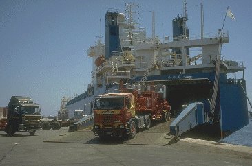 Ultimately
Halliburton and IDM were the successful vendors for the primary 15,000 HHP kill plant and
the mud/water/gunk plant respectfully. All of this equipment was sourced in the United
States. Air freight of the IDM and Halliburton equipment was not an economical option.
Ocean freight was possible as the relief wells had 45+ days to reach intercept points. The
M.V. Krohnstadt (Russian built and staffed "roll-on, roll-off") was contracted.
The ship traveled on the 16 June. There was only 6 days given to Halliburton and IDM to
mobilize equipment to the dock for loading. IDM in particular was able to source and
construct the mud plant in record time. Four IDM men remained on board the ship to
complete work on the mud plant as the ship traveled directly to Middle East. In addition
to the kill equipment, cement grade Wyoming bentonite, for the gunk, and GCA-21 polymer
was also loaded on the Krohnstadt.
Ultimately
Halliburton and IDM were the successful vendors for the primary 15,000 HHP kill plant and
the mud/water/gunk plant respectfully. All of this equipment was sourced in the United
States. Air freight of the IDM and Halliburton equipment was not an economical option.
Ocean freight was possible as the relief wells had 45+ days to reach intercept points. The
M.V. Krohnstadt (Russian built and staffed "roll-on, roll-off") was contracted.
The ship traveled on the 16 June. There was only 6 days given to Halliburton and IDM to
mobilize equipment to the dock for loading. IDM in particular was able to source and
construct the mud plant in record time. Four IDM men remained on board the ship to
complete work on the mud plant as the ship traveled directly to Middle East. In addition
to the kill equipment, cement grade Wyoming bentonite, for the gunk, and GCA-21 polymer
was also loaded on the Krohnstadt.
The ship arrived in country on 6 July and was unloaded with the limited port equipment available. The total length of the journey from port of Houston to Middle East took a total of 21 days. A total of 5 days were required to move equipment from the port to the well site. .
The cement plant was contracted to Dowell and utilized local equipment with the exception of 2 Halliburton RCM mixers. The gunk plant was made-up primarily of NOWSCO equipment that was left over from the second kill attempt. The silicate plant consisted of cementers from several local venders.
 Kill Plant Installations. Hyperlinked
figure, shows a basic aerial view of the blowout and relief well locations (not to
scale), with relative positions of water lagoons, mud plant, and pipelines. Ultimately all
of the rigs were dependent on the water plant and lagoons. The water plant consisted of a
generator powering two 5x 6 pumps charging a 13-3/8" line to the mud plant. Water
could then be transferred via the 7" ring loop between the rigs after water was
pumped to RW1 or water could be directed directly into the 7" loop from the mud plant
or directly off the 16".
Kill Plant Installations. Hyperlinked
figure, shows a basic aerial view of the blowout and relief well locations (not to
scale), with relative positions of water lagoons, mud plant, and pipelines. Ultimately all
of the rigs were dependent on the water plant and lagoons. The water plant consisted of a
generator powering two 5x 6 pumps charging a 13-3/8" line to the mud plant. Water
could then be transferred via the 7" ring loop between the rigs after water was
pumped to RW1 or water could be directed directly into the 7" loop from the mud plant
or directly off the 16".
Halliburton Kill and Dowell Cement Plants. Hyperlinked figure, shows an aerial view of the Halliburton kill plant and Dowell cement plant behind relief well # 1. Both of these plants were rigged up and power tested in 5 days. The power test indicated 16,800 HHP was available, 1800 HHP more than originally advertised. The hyperlinked figure shows the hook-up to the wellhead and drillpipe. 4000 HHP was isolated from the total kill HHP to pump mud or cement down the drillpipe switchable by opening or closing wheel valves. 15 ppg mud, gel mud or water was delivered to the system from the central mud plant either directly to the suction header of the two blender trucks or into 2 x 500 bbl buffer tanks. The blender trucks (centrifugal pumps) 100 % redundancy, then charged the suction manifold (30 - 50 psi). The high pressure pumps then discharged into 3 x 4" ID, 6" OD lines going to the annulus of relief well # 1. Two 3" lines came off one of the 4" lines and connected to a pump-in tree on the drillpipe. Flow rates were measured on the low pressure manifold and summed for total flow. 8" flow meters were used for high flow rates and 4" flow meters were used for low flow rates.
 Central Mud/Gunk Plant. This plant was arranged in 4
modules. Each module consisted of 6 x 500 bbls frac tanks commonly manifolded and serviced
by a 350 bbl mud mixing skid. Two 5x6 mixing centrifugals were used to mix and transfer
mud to frac tanks. One 6 x 8 centrifugal was used to circulate the frac tanks and
supercharge the 12" ID suction line. This equipment was arranged on a sloping pad
with all frac tanks and suction lines pointed downhill for gravity assisted drainage. It
required 3 days to assemble the mud plant. The plant was pre-commissioned with water and
flushed out before mud and gunk mixing began. Cement was not mixed with the gunk until the
day before the kill. Click
here to see picture of mud plant.
Central Mud/Gunk Plant. This plant was arranged in 4
modules. Each module consisted of 6 x 500 bbls frac tanks commonly manifolded and serviced
by a 350 bbl mud mixing skid. Two 5x6 mixing centrifugals were used to mix and transfer
mud to frac tanks. One 6 x 8 centrifugal was used to circulate the frac tanks and
supercharge the 12" ID suction line. This equipment was arranged on a sloping pad
with all frac tanks and suction lines pointed downhill for gravity assisted drainage. It
required 3 days to assemble the mud plant. The plant was pre-commissioned with water and
flushed out before mud and gunk mixing began. Cement was not mixed with the gunk until the
day before the kill. Click
here to see picture of mud plant.
Gunk and Silicate HHP Plant. Hyperlinked figure, shows and aerial view of gunk and sodium silicate (diesel/water) plants located behind relief well # 2. The two plants were totally independent with gunk plant plumbed to pump only in the annulus and the other to pump only in the drillpipe. The gunk plant was setup similar to the Halliburton plant. Gunk would be transferred from the central plant to the two 500 bbl buffer tanks where a centrifugal would charge the suction manifold. The gunk HHP plant tested a total of ˜ 4500 HHP using 8 pumps of various designs. The silicate plant was tested to pump diesel, water or silicate on demand down the drillpipe. The rig pumps could be utilized to pump water down the drillpipe or annulus in addition to the cementing pumps. There was 1 cementing pump attached to the annulus for low pump rate of water < 1 bpm, during the cementing phase of the kill operation. A computer unit was set to monitor flow rates and pressures on both the annulus and drillpipe.
Communication and Drills. A communications system was put in place between the two relief well sites and the Mud Plant. Radio communication was used to coordinate at each of the three sites and water plant. The communication system between the HOWCO control van , NOWSCO van and Mud Plant Office was a hard lined phone.
To get all personnel trained in proper use of phone and radio systems and to gain familiarity with the kill program "Kill Drills" were held. These drills consisted of men in position with equipment fired up at times running through various options outlined in the prepared decision trees. A total of 5 of these drills were held in preparation for the kill. The drills were handled without any pumping but valves were manipulated where possible and the drill ran for up to 2 hours. After each drill the job would be criticized by all parties and steps changed to get a smoother operation.
Downhole Pressure Gauge. Relief well # 2 would be the primary monitor well for down hole pressure using the drillpipe as a dead string. Due to low flowing BHP, however, a hydrostatic column of water would be too heavy to measure a surface pressure. This was the reasoning for having diesel as the primary drillpipe monitoring fluid. To eliminate all uncertainty as to the flowing BHP a decision was made to lower a standard wireline pressure gauge on a landing ring at the bottom of the drillpipe in relief well # 2. The surface readout pressure would then be sent to the HOWCO computer van to control the kill job.
Kill Operational Plan. A detailed kill operational plan including a decision tree and procedural flowchart was designed to guide the control team through the various possibilities and options available as the kill progressed. The basic plan was to first attempt to kill the well dynamically with 2000 bbls of gel mud. If at the end of this operation the BHP indicated this approach may be successful water would be pumped for several hole volumes followed by cement. If it did not appear to be successful 15 ppg mud would follow the gel mud. If the 15 ppg mud kill was successful with less than 2500 bbls pumped it would be followed by cement. If not the gunk kill would be initiated. If the gunk kill was successful it would be followed with cement. If not the sodium silicate and cement option would be attempted as a last resort. Click here to see decision tree flowchart for kill operation.
If all options failed the flood well would be completed while the second kill attempt was planned based on data learned from the first.
Relief Well Operations. Relief well # 1 was spudded on May 24. Relief well # 2 was spudded on June 2. Relief well # 3 was spudded on June 9. The planned dual intersection for relief wells 1 and 2 was August 6. Relief well 1 would drill a 8-1/2" pilot hole with a diverter system through the surface permeable formations to ˜ 300 m and then drill rotary 12-1/4" hole to the KOP and directional 12-1/4" hole to the 13-3/8" casing point. The 12-1/4" hole would then be open up to 17-1/2". Relief well 2 would drill 17-1/2" hole to the kick-off point, then 12-1/4" hole to the casing shoe. The directional section would then be opened up to 17-1/2". The timing of the 3 wells was such that they should converge at the 9-5/8" casing point within a couple of days of each other. Relief well # 1 was planned to intersect first followed by relief well # 2 two or three days later. Relief well # 3 would not proceed to the flood target and set casing until at least one intersection was made. This was necessary to avoid magnetic interference with the homing-in tools.
Relief Well Ranging and Intersection Results.
Ranging began with Well-124 run 1 on 16 July at 2710m MD, 50m from the Well-123 surveyed position. This was a "safety" run. While 50m was beyond the expected detection range, the radius of position uncertainty for the Well-123 was within the expected maximum range. Hole problems prevented the Wellspot tool from reaching bottom; the first reading was at 2660m. There were high formation and wireline background signals. Any target signal was smaller than the background and could not be detected.
Well-124 run 2 on 18 July at 2767m MD also could not reach driller's TD; first reading was 2747m. Again high formation and wireline background signals prevented detection of what was anticipated to be a small target signal.
Well-124 run 3 on 21 July at 2835m MD (9 5/8" casing point). Once again Wellspot could not reach driller's TD, first reading was 2820m. This run was also inconclusive. An increased signal intensity was encouraging and possibly from the target well, however the additional signal could easily be attributed to the background formation and wireline signals.
Well-125 run 1 on 27 July detected the target casing at an estimated 7-12 meters and 0-20� right of highside. Subsequent data indicates the range was 12-14 meters and about 20� right of highside. A solenoid survey was run on the same descent to tie Well-125 and Well-126 together. At 2670m TVD Well-126 was found 12� 1 meters from Well-125 on an azimuth of 95� , about 4 meters farther away than the gyro surveys indicated.
Well-126 run 1 on 28 July at 3096m MD was inconclusive. This well was approaching the Well-123 deeper than the other relief wells. The target signal was greatly reduced by pipe end effects and overwhelmed by background signals. No further runs were made on this well; its relative position to the other relief wells and the target was defined by the solenoid survey from Well-125.
Well-124 run 4 on 29 July at 2917m MD detected the Well-123 at 12� 3 meters and 25� 10� right of highside. A solenoid survey on the same descent found the Well-125 27� 2m away on an azimuth of 48� at 2675m TVD, within about 2 meters of the gyro surveyed positions.
Well-124 run 5 on 30 July at 2950m MD found the Well-123 at 8� 2 meters. Modeling was confirmed by triangulation of the target with Well-125. Actual separation at this depth was approximately 5 meters based on the intercept location. Well-125 run 2 on 30 July at 2979m MD located the Well-123 at 10� 3m and 10� 10� left of highside.
Well-124 run 6 on 31 July at 2977m MD found Well-123 1.1 meters away and 35� 5� right of highside. The Wellspot Gradient Tool was used on this run. The magnetic field gradient-based distance measurement had an effective range of approximately 5 meters. Normalized Intensity was reduced from previous runs, probably due to changing flow conditions in the blowout, which were evident at the surface. A second solenoid survey to Well-125 was taken on the same descent to tie the relief wells together with better accuracy now that they were closer to each other. At 2742m TVD Well-125 was 13.5� 1 meter from Well-124 on an azimuth of 44� . Communication with Well-123 was established after drilling ahead with a rotary assembly.
Well-125 run 3 on 1 August at 3004m MD. The target appeared to be 5-10 meters away on an azimuth of 216� . This was in disagreement (primarily in direction) with the location found in 124 and interpreted as a strong directionally biased formation signal perturbing the target signal. The well was drilled toward the location confirmed by Well-124.
Well-125 run 4 on 3 August at 3020m MD. Distance was measured with the Wellspot Gradient Tool as 2.3 meters to the 123 on an azimuth of 22� 10� left of highside. 125 was expected to pass slightly north of 123.
Well-125 run 5 on 4 August at 3033m MD. This run was inside non-magnetic heavy weight drillpipe after drilling to the expected intersection depth without establishing communication. Normalized Intensity was reduced 85% in the drillpipe. 125 was just passing north of 123, approximately 35cm edge to edge. Acidizing established communication.
Solenoid surveys: A solenoid tool was used to tie Well-124 to Well-125 and Well-125 to Well-126. These data were used to adjust the relief well relative positions and use triangulation to locate the target, based on the assumption that Wellspot direction data is more precise than distance interpretation using the intensity. The solenoid survey was the only method to tie the formation flood well, Well-126, to Well-125 and the target.
Solenoid survey results:
| Depth, mTVD | 125 fr 124 | Direction |
Well-125moveN | Well-125moveE |
| 2675 | 27� 2m | 48� 3� | 1.9m | -1.0m |
| 2742 | 13.5� 1m | 44� 3� | 1.3m | -0.8m |
| Depth, mTVD | 126 fr 125 | Dir. | Well-126moveN | Well-126moveE |
| 2670 | 12� 1m | 95� 3� | -2.3m | 4.1m |
Conclusions: The Wellspot active excitation method was successful in the presence of a 100% insulating fluid flow. Pipe contact with the borehole wall was sufficient, however signal intensity was reduced more than 50%. Actual initial detection range was about 25 meters from Well-124 at the 9-5/8" casing point, run 3. The run was called inconclusive because the unusually high formation signal was several times the target signal. Subsequent runs showed the intensity increase was in fact due to the target and not formation signal.
Whether or not the pipe had been completely severed when shot at 2880m added uncertainty to interpreting distance to the blowout. The location of the effective bottom of the pipe (electrically) affects modeling of the Wellspot intensity data. By run five in Well-124 it became evident the pipe was continuous to 2936m.
There was a large formation signal component to the Wellspot measurement in all three relief wells. This was probably due to strongly oriented formation fractures. Well Well-125 exhibited the highest formation signal and was said to be drilled on an azimuth close to the fracture direction, which may also account for the high ROP experienced in Well-125. The formation signal is deduced where the target signal can be assumed small and the wireline background signal well modeled. The formation signal magnitude in 124 at 2500m md was approximately 65 uA/m/A; the target well signal did not approach that magnitude until Well-124 reached almost 2900m md.
The formation signal perturbed the Wellspot direction measurement significantly in Well-125, distorting the apparent direction to the target as much as 15� left at 10m proximity. Interpretation of the target distance was affected in Well-124 run 5 when triangulation, using direction from 124 and 125, made the apparent distance 8 meters rather than the actual 5 meters. Run 3 interpretation in well 125 was based on the blowout location from 124 and the solenoid measurements that tied 124 to 125 because of this direction distortion. Well 124 did not suffer distortion similar to 125 because it was perpendicular to the fracture orientation.
It is not uncommon to operate Wellspot a short distance below casing, with the excitation electrode well inside casing. That was not possible in either Well-124 or Well-125, probably due to an insulating cement sheath. It was necessary to change over to a shorter bridle/electrode distance to get the electrode out of the 9 5/8" casing. Click here to see final alignment before intersection on Relief Well # 1.
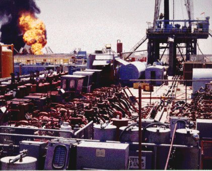
Final Kill Operation
Establishing Communication. The initial intercept was made by RW1 (Well 124) on August 2. Break through required pressuring up on the wellbore to break through a few centimeters of hard limestone. Acid was pumped after break through to assure good communication. Break through in RW2 (Well 125) required five acid jobs of 28% HCL of 10, 20, 20, 40 and 40 bbls on August 4. The bit was spaced adjacent to the point of closest approach estimated at between 20 and 60 cm. These intercepts were made in dense limestone with very low permeability. Water was pumped at >20 BPM with rig pumps after communication was made to confirm good communication.
Strip Up and Surface Hook-up. Drill pipe was stripped up in RW1 inside the 9-5/8" casing shoe. This was not done in RW2 in an attempt to get the SRO BHP gauge as deep as possible. Annular pump-in lines were already hooked up and tested, the drill pipe pump -in lines were laid out and only needed final hook-up and testing. No blast joint was required as velocity through the three 4-1/16" opening was low at 85 BPM with 15 ppg mud. The SRO pressure gauge was run inside the drillpipe in relief well 2 drillpipe and seated in a landing ring. The cable was slacked off 1m. The initial flowing BHP read was 2620 psi.
 Ramp Up for Dynamic Kill.
BY 14:32 Hours rate had peaked at 94 BPM with the HOWCO pumps with a surface
pressure of 3200 psi. The annulus rate on relief well # 2 was increased to 22 bpm with the
rig pumps. The diesel rate was 8 bpm. Combined with the diesel and water rate down RW2,
the total rate was 120 BPM. Dynamic kill was achieved in less than 12 minutes and with
less than 1500 bbls of fluid. Kill was maintained by holding the equivalent of a water
gradient as a minimum pressure.
Ramp Up for Dynamic Kill.
BY 14:32 Hours rate had peaked at 94 BPM with the HOWCO pumps with a surface
pressure of 3200 psi. The annulus rate on relief well # 2 was increased to 22 bpm with the
rig pumps. The diesel rate was 8 bpm. Combined with the diesel and water rate down RW2,
the total rate was 120 BPM. Dynamic kill was achieved in less than 12 minutes and with
less than 1500 bbls of fluid. Kill was maintained by holding the equivalent of a water
gradient as a minimum pressure.
Ramp-down, Maintain Kill. Pumps were ramped down while maintaining a water gradient equivalent pressure down hole. Ultimately pumps were slowed to 35 BPM while holding a water gradient. A large amount of water was pumped to flush out ant hydrocarbons and to allow any bypassed hydrocarbons to lubricate out. A total of 8000 bbls of water were pumped.
Cementing.
Cementing operation started at 17:00. Cementing went as planned with kill
maintained by pumping down RW1 annulus with water while loading DP with cement. As cement
rate was increased the water rate was decreased until cement rate was at 30 BPM. Once
cement was exiting drill pipe the water rate in the annulus was slowed to <0.5 BPM.
Pumping rate on RW2 was slowed to <0.5 BPM. Cement was initially pumped at 30 BPM until
first signs of squeeze was seen. Rate was slowed to 5 to 6 BPM to attempt to get higher
squeeze pressures. Maximum squeeze pressure was 10 ppge. A total of 2440 bbls of cement
was pumped. Cement density was 15.8 to 16.3 ppg. The cement in the final stage was
densified to 16.3 ppg to get faster setting time.
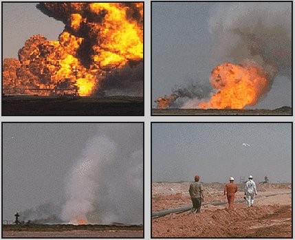
Click here to see sequence of photos taken
during kill.